微分的四层理解

一 微分是无穷小？

物理人喜欢把微分看做是一个很小的量，这在计算时总是很方便的，但是给人一种不严谨的感觉。

实际上，它确实不严谨，第二次数学危机就是因此产生的。

严谨性与易懂性永远是互补的。把微分看做无穷小，迎合感性的胃口，却无法通过理性的审查。

二 微分是线性函数

我喜欢把微分看做一个机器，例如

$f:f(x,y)=x^2+2y^2$

在 $(1,1)$ 处的微分

它就是这样一个机器：

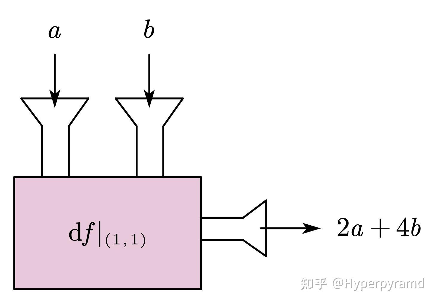
它接受两个数，吐出一个数。

写出来就是这样：

$\mathrm{d}f|_{(1,1)}(a,b)=\frac{\partial f}{\partial x}\bigg|_{(1,1)}a+\frac{\partial f}{\partial y}\bigg|_{(1,1)}b=2a+4b$

由于每一点的偏导可能不同，所以如果说某一点的微分是一个机器，那么，微分就是机器构成的海洋。

你可能还注意到了这个机器是“线性的”，它不过就是 $\mathbb{R}^2$ 到 $\mathbb{R}$ 的线性映射。

线性代数的知识告诉我们，线性函数的集合可以构成线性空间。换言之，线性函数自己就是个“矢量”，是可以加减数乘的。

回到上面的比喻，就是说，我们可以把两个机器加起来： $\mathrm{d}f|_p+\mathrm{d}g|_p$ ，

也可以将一个机器变为原来的 $\lambda$ 倍大： $\lambda \cdot \mathrm{d}f|_p$ 。

下标 p 表示在 p 点的微分。

把机器加起来是什么意思呢？举个例子，若

$\mathrm{d}f|_p(a,b)=2a+4b,,, \mathrm{d}g|_p(a,b)=a-b$ ，

则 $\mathrm{d}f|_p(a,b)+\mathrm{d}g|_p(a,b)=3a+3b$ 。

这很像是两个矢量的相加： $(2,4)+(1,-1)=(3,3)$ 。

实际上，它们就是矢量。是的，你没听错，微分是矢量（场）。

三 微分是对偶矢量场

3.1 切空间

如果你想要在一个弯曲的面上研究微分，那么你就需要重新定义一些概念。比如，微分是线性的，可是流形是弯曲的，所以我们需要在这弯曲中定义一个线性的东西出来。这个线性的东西就是切空间。

顾名思义，切空间就是一个曲面在某一个点处的切面。但是要怎么定义它呢？这里的弯曲并不是嵌在另一个空间里的弯曲，而是空间本身的弯曲，这种弯曲是内禀的。我们不能像古典解析几何那样去求切面方程。

我们换一个思路：

首先，它是线性的，也就是说它是一个向量空间。

向量空间就是一个配备了数乘的阿贝尔群。具体地说，它里面的元素（称为矢量）满足如下性质：
（1）矢量的加法交换律
（2）矢量的加法结合律
（3）矢量的加法有单位元(类似于零)
（4）矢量的加法有逆元(类似于相反数)
以上四个性质表明线性空间对于矢量加法而言是一个阿贝尔群。
（5）数乘有乘法单位元
（6）数乘的乘法结合律
（7）数乘的乘法分配律（对标量分配）
（8）数乘的乘法分配律（对矢量分配）

向量空间不必是 $\mathbb{R}^n,,\mathbb{C}^n$，只要一个集合里定义了加法和数乘运算且满足以上性质，这个集合就是一个向量空间。

我们可以定义这样一个向量空间，它其中的元素是光滑函数的集合到实数域的线性映射：

$v:\mathcal{F}_M\rightarrow\mathbb{R}$ 满足
（1）$v(\lambda f+\mu g)=\lambda v(f)+\mu v(g)$ （线性律）
（2） $v|_p(f\cdot g)=f|_p\cdot v(g)+g|_p\cdot v(f)$ （莱布尼茨律）
其中 $\mathcal{F}_M$ 是微分流形 $M$ 上所有光滑函数构成的集合。

可以证明， $v$ 的集合可以构成向量空间。

别看这个定义这么复杂，实际上就是对一个函数在某一点求方向导数。

以二元函数为例，我们显式地写出 $v$ 的一个实例： $\left(a\frac{\partial}{\partial x}+b\frac{\partial}{\partial y}\right)\bigg|_p$

如果以 $(\frac{\partial}{\partial x}\bigg|_p,\frac{\partial}{\partial y}\bigg|_p)$ 为基，那么它的坐标就是 $(a,b)$ 。

这个线性空间就是流形 $M$ 上点 $p$ 处的切空间，记作 $T_pM$ 。

以上所有操作都是在某一点 $p$ 的，每一点都长出了一个切空间。你可以想象成弯曲面上的每一点都长出了一个切平面。

3.2 余切空间

刚才介绍了切空间 $T_p M$ 。我们现在把切空间的对偶空间 $T_p^*M$ 叫做余切空间。

某一点的微分正是余切空间中的元素。换言之，某一点的微分是一个余切矢量。

对偶空间中的元素（余切矢量）是线性泛函，能把原空间中的元素映射成一个数。这正是我们之前所说的机器：

只不过现在的输入应该是切空间中的元素 $\left(a\frac{\partial}{\partial x}+b\frac{\partial}{\partial y}\right)\bigg|_p$ 。

我们说过，微分是机器的海洋。因此余切矢量的海洋（也就是微分）可以叫做余切矢量场。

在数学中，微分（余切矢量场）有一个酷炫的名字，叫做余切丛的截影。详见

https://zhuanlan.zhihu.com/p/629852598

说了这么多抽象废话，下面来定义一下：

流形 $M$ 上某一点 $p$ 处的微分是这样一个线性泛函，它作用到切空间的元素 $v|_p\in T_pM$ 上，得到 $\mathrm{d}f|_p(v|_p)=v|_p(f)$

再举一个更显式的例子，以二元函数为例：

$\mathrm{d}f|_{p}:\mathrm{d}f|_{p}(v|_p)=v|_p(f)= \frac{\partial f}{\partial x} \bigg|_{p} a+\frac{\partial f}{\partial y}\bigg|_{p}b$ ，其中 $v|_p=\left(a\frac{\partial}{\partial x}+b\frac{\partial}{\partial y}\right)\bigg|_p$

四 微分是 Jacobian 矩阵刻画的线性映射

到目前为止，我们讨论的都是到达域为 $\mathbb{R},\mathbb{C}, \cdots$ 的函数。如果到达域可以是 $\mathbb{R}^2, \mathbb{R}^3,\cdots$ 呢？

例如 $\bm{f}:\mathbb{R}^n\rightarrow\mathbb{R}^m$ 。

此时，可以把 $\bm{f}$ 看成 m 个函数：

$f_i:\mathbb{R}^n\rightarrow\mathbb{R},,,i=1,\cdots,m$

那么就有

$\begin{bmatrix}\mathrm{d}f_1 \\ \mathrm{d}f_2 \\ \vdots \\ \mathrm{d}f_m \end{bmatrix}= \begin{bmatrix} \frac{\partial f_1}{\partial x_1}&\frac{\partial f_1}{\partial x_2}&\cdots&\frac{\partial f_1}{\partial x_n} \\ \frac{\partial f_2}{\partial x_1}&\frac{\partial f_2}{\partial x_2}&\cdots&\frac{\partial f_2}{\partial x_n} \\ \vdots&\vdots&\ddots&\vdots \\ \frac{\partial f_m}{\partial x_1}&\frac{\partial f_m}{\partial x_2}&\cdots&\frac{\partial f_m}{\partial x_n} \end{bmatrix}\begin{bmatrix}\mathrm{d}x_1 \\ \mathrm{d}x_2 \\ \vdots \\ \mathrm{d}x_n \end{bmatrix}$

其中 $\begin{bmatrix} \frac{\partial f_1}{\partial x_1}&\frac{\partial f_1}{\partial x_2}&\cdots&\frac{\partial f_1}{\partial x_n} \\ \frac{\partial f_2}{\partial x_1}&\frac{\partial f_2}{\partial x_2}&\cdots&\frac{\partial f_2}{\partial x_n} \\ \vdots&\vdots&\ddots&\vdots \\ \frac{\partial f_m}{\partial x_1}&\frac{\partial f_m}{\partial x_2}&\cdots&\frac{\partial f_m}{\partial x_n} \end{bmatrix}$ 就是 Jacobian 矩阵。

实际上，微分就是 Jacobian 矩阵所表示的线性映射。下面我们来详细解释一下。

对于一元函数，Jacobian 矩阵就是导数。

虽然我们习惯把导数看做斜率，但是我们现在不妨换个看法：如果你把一元函数的作用看作是数轴的拉伸，那么导数就是局部的伸缩比率。这样的好处是容易推广到多元函数。

因为，对于多元函数，你通常很难像一元函数那样做出一条曲线来表示函数。所以，作为一种替代方法，你可以把多元函数看做是空间的拉伸，例如 f: R^2→R^2。你可以想象 R^2 的每一点都被 f 拉到了新的一点。

如果你放大这个拉伸的局部，它看起来也像一元函数的情形那样，是线性的——平行等距的线被拉伸成平行等距的线。

而我们所说的微分，正是这个局部的线性映射！这个线性映射的矩阵就是 Jacobian 矩阵。

Khan Academy 的 Multivariable Calculus 课程的第 71-72 集有更详细的解释：

https://www.youtube.com/watch?v=bohL918kXQk
如果显示网络错误，你也可以看 b 站的搬运：

https://www.bilibili.com/video/BV1NJ411r7ja?from=search&seid=11489752606099978202