【量光实验杂谈·三】量子态层析
Quantum State Tomography(量子态层析)
Quantum state tomography(量子态层析)就是根据【对量子态系综的测量结果】反推【量子态】的过程。它的 formulation 非常简单,具体如下:
已知一系列测量算符 ${\Pi_1,\cdots,\Pi_n}$ 及其对应的测量概率 $p_k=\operatorname{Tr}[\rho \Pi_k]$ ,求量子态 $\rho$ 。
换句话说,在 $p_k=\operatorname{Tr}[\rho \Pi_k]$ 这 n 个公式里面,已知 $p_k$ 和 $\Pi_k$ ,求 $\rho$ 。
反过来,如果已知 $\rho$ 和 $p_k$ 求 $\Pi_k$ ,那么就叫 Detector tomography。不过这不是本篇文章的内容。
为什么要关心 state tomography?因为我们想要知道实验上制备的量子态具体长啥样。方法就是 state tomography。
从公式 $p_k=\operatorname{Tr}[\rho \Pi_k]$ 中可以看出,如果 $\rho$ 有 $n$ 个自由度,那么我们也至少需要 $n$ 个 测量算符,而且这些测量算符之间还要“相互独立”,这个条件叫做 tomographical completeness 或者 informational completeness。
为什么叫“层析”(tomography)?
State tomography 之所以叫“tomography”,是因为连续变量光子态的 tomography 和 医院里做的 CT(Compute tomography)真的很像。CT 是已知各个角度的投影图像,重建三维图像,而连续变量光子态的 tomography 就是已知各个角度的投影图像,重建 Wigner function。后者是一种“二维图像”。
当然,用离散变量也是可以理解的,因为(von Neumann)测量无非就是投影,而 tomography 就是根据测量到的投影来重建原量子态。
总之,tomography 之所以叫 tomography,就是因为它是一个根据投影来重建整体的过程。
一个 Qubit 的 State tomography
一个 qubit 的密度算符只有三个自由度(Bloch vector),所以理论上只需要三个测量算符就可以了。例如可以选择 ${(\mathbb{I}+X)/2,\,\, (\mathbb{I}+Y)/2,\,\, (\mathbb{I}+Z)/2 }$ 这三个测量算符(其中 $X,Y,Z$ 是泡利矩阵)。它们在 Bloch 球上对应 X, Y, Z 三个轴,相当于分别测量 Bloch vector 的 x, y, z 分量。
但问题是,在实验上,我们不是直接测量概率,而是测量结果的计数。我们如果想要知道概率 $p_Z=\operatorname{Tr}[\rho (\mathbb{I}+Z)/2] = \langle0|\rho|0\rangle$ ,就必须要利用计数 $p_Z=\frac{N_Z}{N_Z+N_{-Z}}$ ,而测量 $N_{-Z}$ 又需要新的一个 测量算符 $(\mathbb{I}-Z)/2$ 。
更一般地说,由于我们测量的是计数,需要 normalization,所以实际需要的测量算符数量总是比理论需要的多一个。而 N 个 qubit 的密度算符的自由度是 $4^n-1$ ,再加一刚好就是 $4^n$ 了。
对于 n=1 而言,我们就需要 4 个测量算符。这也是最早的光子态 tomography 文章[1]所采用的方法。
好了,withour further ado,我们来仔细研究一下一个 qubit 的 tomography,这对后面推广到多个 qubit 有帮助。
一个 qubit 的密度算符是 $\rho = \frac{\mathbb{I}+xX+yY+zZ}{2}$ ,对其进行 tomography 就是要求解 $x, y,z$ 。正如前文所说,我们选取四个测量算符: ${(\mathbb{I}+X)/2,\,\, (\mathbb{I}+Y)/2,\,\, (\mathbb{I}+Z)/2, \,\,(\mathbb{I}-Z)/2 }$ 。那么测量到的计数分别为
$N_{X} = N p_X = N \operatorname{Tr}[\rho \frac{\mathbb{I}+X}{2}] = N\frac{1+x}{2}$
$N_{Y} = N p_Y = N \operatorname{Tr}[\rho \frac{\mathbb{I}+Y}{2}] = N\frac{1+y}{2}$
$N_{Z} = N p_Z = N \operatorname{Tr}[\rho \frac{\mathbb{I}+Z}{2}] = N\frac{1+z}{2}$
$N_{-Z} = N p_{-Z} = N \operatorname{Tr}[\rho \frac{\mathbb{I}-Z}{2}] = N\frac{1-z}{2}$
联立这四个方程,我们就能求出 $x,y,z,N$ 四个未知数。
OK,完事了,就是这么简单。
极大似然估计
等等,真有这么简单吗?敏锐的同学会发现,密度算符有正定性的要求,但是上面的求解过程没有任何一步能够确保正定性。
实际上,如果按照上面的步骤求解,是完全有可能解出非正定的密度算符的。换句话说,会求解出“非物理”(non-physical)的结果。
这是因为实验数据是有误差的,这种误差在某些情形下会导致非物理的结果。
注意,不是实验系统不理想导致的误差,而是量子统计本身的误差,或者说 fluctuation。例如,对于 coherent state,其计数分布是泊松分布,方差等于均值。在时间有限不能获取很多数据的时候,相对误差 $\frac{\Delta N}{N}=\frac{1}{\sqrt{N}}$ 会比较大。
有同学可能马上就会说:那我们再给结果加一个约束不就行了?在这个例子里,我们只要要求 $|x|,|y|,|z|\le1$ 就可以保证正定性了。
但问题随之而来:加了约束以后,非正定的情形就直接变成无解了。
OK,既然无解是由误差导致的,那么我们可以退而求其次,把问题从【解方程问题】变成一个【拟合问题】。
什么是拟合问题?我们知道,两点确定一条直线。而在数据点本身误差较大的时候,我们需要很多个点,这些点几乎一定不在一条直线上,此时直线方程无解。
虽然无解,但是我们可以拟合呀!用最小二乘法就可以了!
那么最小二乘法是从哪里来的?答案就是极大似然估计(Maximum Likelihood Estimation,MLE)。
极大似然估计的思想就是找到这样一条直线,使得这条直线(在诸多直线中)是最有可能产生我们所测量到的点的那一条直线。具体的执行方式就是设置一个似然函数,它的自变量是直线的参数,且它的函数值是在该直线的前提下,测量到已有结果的概率。然后整个问题就变成了一个优化问题:找到似然函数的最大值及其对应的直线参数。
在很多情况下,人们把实验误差假设为符合正态分布,那么似然函数就是一个指数形式 $L=e^{-\mathcal{L}}$ ,然后我们会对似然函数取对数并取相反数得到新的似然函数 $\mathcal{L}$ ,然后找新的似然函数 $\mathcal{L}$ 的最小值。这个新的似然函数一般可以被解读为“在假设该直线的前提下,理论测量结果和实际测量结果之间的误差总和”。
以上所有思想都可以照搬到我们的 state tomography 中。我们可以设置一个似然函数,其自变量是正定矩阵 $\rho$ 的自由度,其函数值是量子态为 $\rho$ 的前提下,测量到所测量到的结果的概率。
下面我们把这些思想转化为算法:
定义合法的密度算符 $\rho(x,y,z)=\frac{\mathbb{I}+xX+yY+zZ}{2}, |x|,|y|,|z|\le1$
定义似然函数为假设量子态为 $\rho$ 时测量到实际结果的概率:
$\begin{aligned} \mathcal{L}(x,y,z) &= P(N_1=n_1,N_2=n_2,\cdots) \\ &= \prod_k \exp\left[-\frac{(n_k-\hat{n}_k)^2}{2\hat{n}_k}\right]\\ &= \prod_k \exp\left[-\frac{(n_k-N\operatorname{Tr}[\rho \Pi_k])^2}{2N\operatorname{Tr}[\rho \Pi_k]}\right] \end{aligned}$
这里采用了连续的正态分布而不是离散的泊松分布,是因为在数量较大时(实验上通常为至少几百个到几千个),正态分布可以很好地近似泊松分布。
将似然函数取为泊松分布也可以,但是结果(见附录)没有那么直观,而且对于计算机来说负担也更大。
为方便计算,对其取负对数,并去掉不必要的常数 $N$,得到:
$\begin{aligned} \mathcal{L}(x,y,z)=\sum_k\frac{\left(p_k-\hat{p}_k\right)^2}{2\hat{p}_k}=\sum_k\frac{\left(p_k-\operatorname{Tr}[\rho(x,y,z)\Pi_k]\right)^2}{2\operatorname{Tr}[\rho(x,y,z)\Pi_k]} \end{aligned}$
此时我们只要求 $(x_0,y_0,z_0) = \underset{|x|,|y|,|z|\le1}{\operatorname{arg\,min}} \mathcal{L}(x,y,z)$ 即可。
这是一个有约束的优化问题。能不能将其转化为无约束的优化问题呢?见下文。
多个 Qubit 的 state tomography
n 个 qubit 的密度算符有 $4^n -1$ 个自由度,此时 Bloch vector 的对应物为 Pauli Correlator:
$\begin{aligned} \rho = \frac{1}{2^n}\sum_{i_1,\cdots,i_n=0}^{3} c_{i_1i_2\cdots i_n} \sigma_{i_1} \otimes \sigma_{i_2} \otimes \cdots \sigma_{i_n} \end{aligned}$
其中 $\sigma_i,\,i=0,1,2,3$ 分别为恒等矩阵和泡利矩阵 $\mathbb{I},X,Y,Z$ 。且 $c_{i_1i_2\cdots i_n}$ 叫做 correlators。
此时我们至少需要 $4^n$ 个测量算符,在这些算符下测量得到计数,然后就可以做极大似然估计了。
此时的态 $\rho$ 可以设置为 $\rho(\mathbf{t})=\frac{T^\dag(\mathbf{t})T(\mathbf{t})}{\operatorname{Tr}(T^\dag(\mathbf{t})T(\mathbf{t}))}$ ,其中
$T(\mathbf{t})=\begin{bmatrix} t_1 & 0 & 0 & \cdots & 0 \\ t_{2^n+1}+it_{2^n+2} & t_2 & 0 & \cdots & 0 \\ t_{2^n+5}+it_{2^n+6} & t_{2^n+3}+it_{2^n+4} & t_3 & \cdots & 0 \\ \vdots & \vdots & \vdots & \ddots & \vdots \\ t_{4^n - 1}+it_{4^n} & t_{4^n - 3}+it_{4^n-2} & t_{4^n - 5}+it_{4^n-4} & \cdots & t_{2^n} \end{bmatrix}$
这是为了保证 $\rho(\mathbf{t})$ 的正定性。
相较于将 correlators $c_{i_1i_2\cdots i_n}$ 作为参数且约束它们的绝对值不大于一而言,T(t) 这种参数化方式的好处是把即将要进行的极大似然估计从有约束的问题变成了无约束的问题(我们对 t 没有任何约束)。
此时的似然函数为:
$\begin{aligned} \mathcal{L}(\mathbf{t})=\sum_k\frac{\left(p_k-\hat{p}_k\right)^2}{2\hat{p}_k}=\sum_k\frac{\left(p_k-\operatorname{Tr}[\rho(\mathbf{t})\Pi_k]\right)^2}{2\operatorname{Tr}[\rho(\mathbf{t})\Pi_k]} \end{aligned}$
测量算符的选取
选取什么样的测量算符才是最好的呢?
一般在偏振编码的光子 qubit 中,我们就简单地使用 H,V,D,A,R,L 这六个投影测量及其组合(它们是很好实现的,只需要使用波片即可)。那么对于 n 个 qubit 而言,此时我们就拥有 $6^n>4^n$ 个投影算符,就够用了。
由于 $(|H\rangle\langle H|, |V\rangle\langle V|)$ 构成一个 POVM, $(|D\rangle\langle D|, |A\rangle\langle A|)$ 构成一个 POVM, $(|R\rangle\langle R|, |L\rangle\langle L|)$ 构成一个 POVM,也就是说 6 个投影测量对应 3 个 POVM,所以我们需要 $3^n$ 个 POVM,实验上就是 $3^n$ 个 measurement settings(所谓 measurement settings 就是波片的角度)。
但是问题来了,还有没有更好的办法可以减少 POVM 的数量,从而减少 tomography 所需的时间?毕竟 $6^n>4^n$ 是冗余的。
从这里开始可以说算是学术界的前沿问题了,可以宣传我们组的一些工作。以后再更吧,哈哈哈。
连续变量光子态的 state tomography
所谓连续变量的光子态(continuous-variable photonic states),就是考虑整个 Fock Space ,而不是只考虑 Fock Space 中的零光子和单光子的子空间。我们之所以关心连续变量,是因为光子本质上是一个谐振子系统,而非一个二能级系统。考虑前者更加自然,也更加符合光子的本质。实际上,我们日常生活中的经典电磁波就是一种连续变量的光子态(即 coherent state)。
单模连续变量光子态可以由准概率分布函数来描述。准概率分布函数有三种,Glauber P-,Husimi Q-,以及 Wigner 函数,它们分别简称 P-,Q-,W- 表示。由于只有 Wigner 函数的边缘分布对应实际观测量的概率分布,所以我们一般考虑 Wigner 函数。
Wigner 函数是什么?
如何理解 Wigner 函数?我们可以先从经典电磁波出发。我们都知道,单模(单一频率)的电磁波可以用复平面上的一个点来描述(即用相图描述)。电磁波的叠加可以直接对应相图中的复数加法(或矢量加法)。
这个所谓的相图表示可以立刻推广到量子力学中。对于量子化的单模经典电磁场,它的相图表示不再是一个无限小的点,而是一个有一定大小的圆。实际上,它是一个复平面上的高斯函数,且该高斯函数的标准差由不确定性原理确定。这个高斯函数就是经典电磁波的 Wigner 函数,其边缘分布对应该 quadrature 的电场强度的概率分布(电场也是可观测量,是有不确定性的)。经典电磁波被量子化之后得到的量子态叫做 Coherent state。
对于一个更一般的量子光场,其 Wigner 函数可以长得奇形怪状,甚至可以取负值。当然,这不意味着我们得到了负的概率——在求边缘分布之后,我们得到的总是非负概率。这是因为这些负值所占据的面积足够小,以至于它们小于不确定性原理所允许的面积,也就是说不确定性原理保证了我们观测不到负概率。
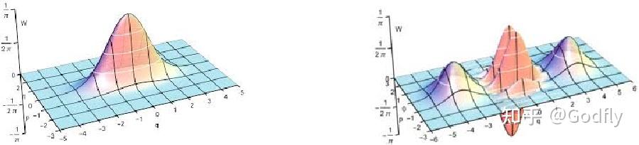
一些有趣的光子态的 Wigner 函数。左图为压缩态,右图为薛定谔猫态。
连续变量光子态的 state tomography 是通过测量 quadrature 来完成的。此时所有的测量算符拥有如下形式:
$\begin{aligned} \Pi_\theta = \frac{ae^{-i\theta}+a^\dag e^{i\theta}}{2} \end{aligned}$
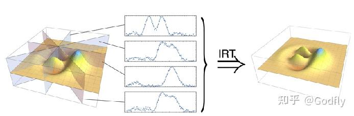
这就是所谓的“quadrature”(不知道中文译名是什么)。形象地来看,它是将整个 Wigner 函数投影到一条直线上,这条直线与 x 轴的夹角为 $\theta$ 。
Quantum state tomography of continuous-variable optical states
量子信息理论告诉我们,如果我们想要(以无限精度)重建 Wigner 函数,我们就需要无限多个 $\theta$ ,即无数个测量算符。当然,我们不需要无限的精度,所以我们只要把 $\theta$ 取得密一些就可以了。例如以 0.01 弧度为步长,从 0 取到 2pi。
得到 quadrature 的概率密度分布函数之后,我们就可以使用逆 Radon 变换重建 Wigner 函数了。这和医院里的 CT 原理完全相同。
至于实验上如何测量 quadratures,很简单,和无线电里一样,将信号与本振进行混频就可以了。这叫做 homodyne measurement。具体来说就是将待测信号和一个激光用一个 beam splitter 混合,然后记录两路输出信号的差值。改变激光的相位就是改变 $\theta$ 。
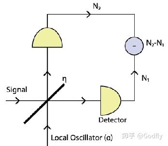
Homodyne Measurement
附录 泊松分布的极大似然估计
泊松分布对应的似然函数为
$ \begin{aligned} \mathcal{L}(\mathbf{t}) &= P(N_1=n_1,N_2=n_2,\cdots) \\ &= \prod_k e^{-\lambda_k} \frac{\lambda_k^{n_k}}{n_k!} \\ &\xrightarrow{-\log} \sum_k (\lambda_k - n_k \log \lambda_k + \cancel{\log n_k!}) \\ &\xrightarrow{\frac{1}{N}} \sum_k(\hat{p}_k(\mathbf{t})-p_k \log \hat{p}_k(\mathbf{t})) \end{aligned}$
其中 $\lambda_k = N \operatorname{Tr}[\rho(\mathbf{t}) \Pi_k]= N \hat{p}_k(\mathbf{t})$ 。
对似然函数求导找极小值,可以发现极小值在 $\hat{p}_k(\mathbf{t}) = p_k$ 时取到。这说明采用泊松分布也是正确的。但是泊松分布的似然函数里有对数,而正态分布的似然函数里都是多项式,后者对于计算机更友好,收敛更快一些。所以我们一般采用正态分布对应的似然函数。
参考
- ^James, D. F. V., Kwiat, P. G., Munro, W. J. & White, A. G. Measurement of qubits. Phys. Rev. A 64, 052312 (2001).