SPDC产生的频率纠缠光,其中的闲置光经过光纤放大器,还与信号光纠缠吗?
SPDC产生的频率纠缠光,其中的闲置光经过光纤放大器,还与信号光纠缠吗?
我们先用极限思维,考虑两个极限:
极限1:放大器的增益等于1,也就是没有任何增益
此时放大器相当于啥也没做,是一个identity channel。那么当然纠缠还是会保持的。(其实也不一定。即使增益为零,也可能引入额外的噪声,我们这里暂且忽略)
极限2:放大器的增益非常大。
假设此时纠缠能够保持,那么我们是可以得到宏观的薛定谔猫态的。但是这样的态实验上基本得不到,因为它早就退相干了。(当然,也有一些例外,例如 bright squeezed states)
那么,介于这两个极限之间,我们可以说,当增益比较小的时候,纠缠能够保持,但是增益比较大的时候(实际上这个“比较大”的数量级估计也就是~10,参考 N00N 态),由于噪声或者退相干,纠缠会消失掉。
下面我们分两种情况讨论,分别是基于 $\chi^{(2)}$ 非线性的参量放大器和基于受激辐射的放大器。
一、基于 $\chi^{(2)}$ 非线性的光放大器
如果这里的光纤放大器是基于 $\chi^{(2)}$ 非线性,即 PDC,参量下转换。PDC 如果用来做光放大,那么也可以叫做 OPA,即光学参量放大。注意,这里的 PDC 要和 SPDC,即自发参量下转换区分开。
假设 SPDC 和 OPA 的 pump 足够强,那么它们的哈密顿量就分别可以写成:
$H_\text{SPDC}=\mathrm{i}\hbar(\hat{a}^\dag \hat{b}^\dag - \hat{a} \hat{b})$
$H_\text{OPA} = \mathrm{i}\hbar(\hat{b}^\dag \hat{c}^\dag -\hat{b}\hat{c})$
其中 $\hat{a}$ 和 $\hat{b}$ 代表 SPDC 的 idler 和 signal 模式上的湮灭算符, $\hat{b}$ 和 $\hat{c}$ 代表 OPA 的 signal 和 idler 模式上的湮灭算符。
那么最终的量子态就是
$|\Psi\rangle = \exp[\mathrm{i}g_\text{2}H_\text{OPA} /\hbar]\exp[\mathrm{i}g_\text{1}H_\text{SPDC}/\hbar] |0,0,0\rangle_{abc}$
其中 $g_1$ 是 SPDC 的增益的对数, $g_2$ 是 OPA 的增益的对数。
最后再 trace 掉 OPA 的 idler 就行了:
$\rho=\operatorname{tr}_c[|\Psi\rangle\langle\Psi|]$
严格的具体计算可能不太好算,做量子信息理论的大佬看到有兴趣的话可以帮忙算一下。另外还要考虑用什么 entanglement measure。PPT 准则肯定用不了,因为这是两个 mode,而不是两个 qubit。
不过也可以猜一下计算过程:盲猜经过 OPA 并且 trace 掉 OPA idler 的这个过程等价于一个 dephasing channel。然后我们再把 SPDC 态在低增益极限下近似为一个贝尔态。此时纠缠程度就直接取决于 dephasing 的强度了,这个强度与 OPA 的增益正相关,并且很可能正比于增益,也就是 $\exp(g_2)$ 。考虑一个 20 分贝的增益,那么纠缠程度会减小 $10^{20/10} = 100$ 倍。
所以经过一通“如算”,我们得到结论:OPA 的增益越大,纠缠程度越小。
二、基于受激辐射的光放大器
以上说的是基于参量下转换的放大器。但最常用的 EDFA 并不是基于 $\chi^{(2)}$ 非线性的,而是基于受激辐射光放大的,和激光的原理一样。
这个时候的哈密顿量就要比 OPA 复杂多了,因为涉及到原子。我们先考虑单模光场:
$H = \hbar\omega a^\dag a + \sum_j \hbar \omega_a \sigma^+_j \sigma^-_j + \hbar \Omega \sum_j (\sigma^+_j a -\sigma_j^- a^\dag)$
其中 $\omega$ 是光场的频率, $\omega_a$ 是原子的能级差, $\sigma^{\pm}$ 是原子能级的升降算符, $\Omega$ 是拉比频率。
这其实就是 Tavis-Cummings model 的哈密顿量。这玩意儿是没有通用解析解的,所以只能做做微扰近似。
经过一顿微扰计算 [1],我们可以得到:
$(\Delta X)^2 = G (\Delta X_{0})^2 + (2 n_{\text{sp}}-1)(G-1) \frac{1}{4}$
其中 $X$ 是光场的任意一个 quadrature,可以理解为电场强度的实部或虚部。 $G$ 是增益。 $n_\text{sp} = \frac{N_2}{N_2-N_1}$ 表示布居数反转的程度, $n_\text{sp}$ 越大,反转程度越低, $n_\text{sp}$ 越小,反转程度越高,最小为 1。
可以发现,EDFA 不仅将输入信号的噪声放大了 $G$ 倍,还额外引入了真空场的噪声,并且将真空场的噪声放大了 $ (2 n_{\text{sp}}-1)(G-1)$ 倍。这就是 ASE,Amplified Spontaneous Emission,即被放大的自发辐射噪声。见下图:
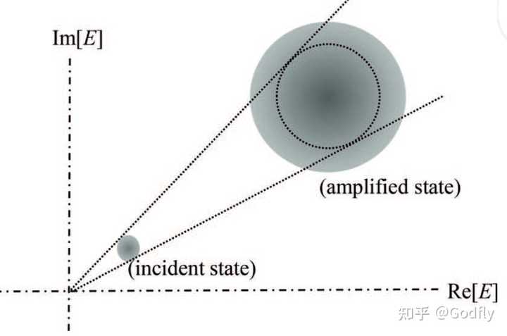
经过 EDFA 的量子态的 Wigner 表示。图源 [1]
以上说的是动力学。这些动力学如何影响纠缠呢?
众所周知,SPDC 得到的 signal 和 idler 是一个纠缠态: $|\Psi\rangle_\text{SPDC} \approx |\text{vac}\rangle + \lambda \int \mathrm{d}\omega_s \mathrm{d}\omega_i f(\omega_s,\omega_i)a^\dag_s(\omega_s) a^\dag_i(\omega_i) |\text{vac}\rangle$ ,其中 $f(\omega_s,\omega_i)$ 是联合频率分布,取决于相位匹配条件和 pump 的线宽(也就是动量守恒与能量守恒条件)。 $|\text{vac}\rangle$ 代表所有模式上的真空态, $\lambda \ll 1$ 表示低增益极限下的 SPDC 的平均光子数,这是实验上常用的情况。
$f(\omega_s,\omega_i)$ 通常不是可分的,即不能被写成 $f(\omega_s,\omega_i) = f_s(\omega_s) f_i(\omega_i)$ 。因此 SPDC 的 signal 和 idler 模式之间呈现出频率纠缠。
既然是频率纠缠,那么我们就要考虑多模情况。为了简单起见,我们只考虑两个频率模式 $\omega = \mu,\nu$ 。那么可以将 SPDC 态写成:
$|\text{vac}\rangle + \lambda (|1\rangle \otimes |0\rangle \otimes |0\rangle \otimes |1\rangle+ |0\rangle \otimes |1\rangle \otimes |1\rangle \otimes |0\rangle)$
其中从左到右四个模式分别是 signal 的 $\mu$ 和 $\nu$ 频率模式和 idler 的 $\mu$ 和 $\nu$ 频率模式。经过 EDFA 放大,得到:
$|0\rangle \otimes |0\rangle \otimes |G,0\rangle \otimes |G,0\rangle +\lambda(|1\rangle \otimes |0\rangle \otimes |G,0\rangle \otimes |G,1\rangle+ |0\rangle \otimes |1\rangle \otimes |G,1\rangle \otimes |G,0\rangle)$
其中 $|G,0\rangle,|G,1\rangle$ 分别表示 $|0\rangle ,|1\rangle$ 经过 EDFA 得到的态。这个东西我实在是不会算。但是我们可以从它们的 Wigner 函数的形状上看出一些端倪。
我们首先看一下 $|0\rangle$ 和 $|1\rangle$ 的 Wigner 函数:
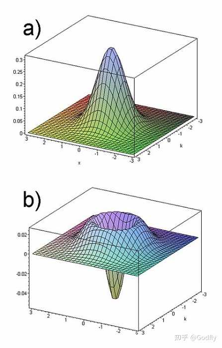
真空态和单光子数态的 Wigner 函数,图源 Wikipedia
它们经过大增益的 EDFA 之后,就会像一张大饼一样,从原点向四面八方摊平,并且还要再加上被放大的自发辐射噪声(ASE),从而单光子数态的 Wigner negativity 应该也会消失。
此时的态已经完全是一个粒子数和相位不确定性都非常大的混态,类似于 thermal state。为什么我 claim 它是一个混态?这是因为在 Tavis-Cummings model 中,最后一步的计算要 trace 掉原子态,这几乎一定会给出一个混态。
在如此大的增益以及粒子数不确定性下, $|0\rangle$ 和 $|1\rangle$ 的区别已经不大,因此应当会有 $|G,0\rangle \approx |G,1\rangle$ 。于是量子态就可以写成:
$ [|0\rangle \otimes |0\rangle+\lambda(|1\rangle \otimes |0\rangle + |0\rangle \otimes |1\rangle)] \otimes (|G,0\rangle \otimes |G,0\rangle)$
前两个模式是 signal 模式,后两个模式是 idler 模式,可见,现在它们不再纠缠,而是可分态。
总结一下就是,EDFA 会将输入信号的噪声放大,并且还额外引入 ASE 噪声,这些噪声会导致量子态变成一个混态。而一般来说,纠缠的纯态变成混态之后,纠缠程度会变低乃至消失。
如果实在非常想刨根问底,可以根据 [1] 中的步骤,在 Tavis-Cummings model 中用微扰论计算一下量子态的演化([1] 中是在海森堡表象下计算,因此只能给出算符的期望值,而不是量子态)。
参考
- Inoue, K. Quantum Noise in Optical Amplifiers. in Optical Amplifiers - A Few Different Dimensions (ed. Choudhury, P. K.) (InTech, 2018). doi:10.5772/intechopen.72992.