量子计量学(Quantum Metrology)简明入门
一、量子计量学介绍
所谓量子计量学(Quantum Metrology),就是利用量子物态的量子性质进行精密测量的学问。
之所以要研究量子计量学,是因为任何物理量的测量精度都由量子力学中的海森堡不确定性原理所限制,这叫做海森堡极限(Heisenberg Limit)。如何逼近以及提升这个极限,就是量子计量学的目标。
当然,日常生活中的大部分测量都不需要达到海森堡极限(例如,称体重)。但是在高精度成像以及各种高精度科学实验中,人们的确早就已经接近了海森堡极限。
引力波:LIGO(Light Interferometer Gravitational-wave Observatory)是人们用来探测引力波的光干涉仪。它能探测到的干涉臂的长度变化达到了 $10^{-19}$ m 的级别,只有一个质子的大小的万分之一,更是光的波长的亿万分之一。在这个疯狂的精度级别下,LIGO 利用了光场的压缩态来降低量子噪声。
当然,量子噪声并非只在 LIGO 这样的极端情况下出现。下面我们给出两个关于成像的例子。
散粒噪声:你一定用过 CMOS 相机。你是否注意过,在环境较暗的情况下,拍出来的照片会有很多噪点?其实它们是由 散粒噪声(Shot noise) 导致的。
什么是散粒噪声?光子激发出来的电子是一个一个的,且这些电子的产生符合泊松分布(产生的时间完全随机),其相对方差反比于平均电子数,这个方差就是散粒噪声。
可见,当电子数量较少的时候,其相对方差会比较大,信噪比(SNR)较低,导致了噪点的出现。
散粒噪声是由粒子数-相位不确定性原理给出的,然而,由于一些历史原因,人们不把它叫做海森堡极限,而是把它叫做散粒噪声极限,或者标准量子极限,并把它与海森堡极限区分开来。
衍射极限:成像精度除了时间上的衡量(即信噪比)以外,还有空间上的衡量,即像素点的个数。如果我们无限增加像素点的个数,有可能达到无限的精度吗?
学过光学的你知道这不可能,因为有衍射极限的存在。
实际上,衍射极限就是一种海森堡极限,因为它对应一种动量-位置不确定性。如果我们需要更准确的位置,衍射极限告诉我们,在不改变波长的前提下,需要增加入瞳(aperture)的大小。从海森堡原理的角度来看,这是因为以不同角度进入入瞳的光子拥有不同的动量,这些动量信息在成像的那一刻丢失了,而丢失的动量信息越多,光子的位置就测量地越准确。反过来,在不改变入瞳大小的前提下,我们需要减小波长,这是因为波长越小,动量越大,相同入瞳所接收到的光子的动量范围也越大。
这些例子都很有趣。希望你 enjoy。当然,更有趣的还在后头呢:人们用什么样的数学工具刻画量子噪声?人们怎样设计量子态以达到海森堡极限?看完这篇文章,你会深入了解这些问题,并且完成对量子计量学的入门。
二、极大似然估计
什么是测量?首先,我们需要给测量下一个定义。注意到,对同一个物理量进行测量总是会以一定概率给出一系列各不相同的结果(无论是经典物理还是量子物理)。我们通常把这些结果的平均值作为最终结果。
可见,测量过程实际上给出了一系列随机变量(即各个单次测量结果),而我们通过构造像平均值这样的统计量(即随机变量的函数)来估计物理量本身。我们把这个统计量叫做估计量(estimator)。
这个估计量本身也是一个随机变量,也有均值和方差。我们将该估计量的取值称为测量结果,其方差称为测量误差。相对误差就是误差除以均值;测量精度就是相对误差的倒数。
到此为止,我们就定义好了测量过程,它本质上是一个参数估计问题:
参数估计:给定一个概率密度函数 $p(\mathbf{x};\theta)$,其中 $\mathbf{x}$ 是测量结果,$\theta$ 是要测量的物理量(它是概率密度函数的一个参数,而非自变量),构造估计量 $\hat{\theta} = \hat{\theta}(\mathbf{x})$ 使得它的均值等于或尽量接近待估计的参数(无偏性),且方差尽可能地小(有效性)。另外,还有一个比较隐蔽的条件:我们要求样本数量越大,估计量就越接近参数的真实值(一致性)。
无偏性:无偏性就是指 $\mathbb{E}(\hat{\theta}(X)) = \theta$,即估计量的均值等于参数的真实值。
有效性:怎样刻画有效性?后面我们会介绍,估计量的方差有 CR 下界:$(\Delta \hat{\theta})^2 \ge \frac{1}{F(\theta)}$,其中 $F(\theta)$ 叫做 Fisher 信息。有效性可以用 $F(\theta)/(\Delta \hat{\theta})^2 \le 1$ 来刻画。当 $F(\theta)/(\Delta \hat{\theta})^2 = 1$,即达到下界时,我们就称该统计量是有效的。
一致性:一致性要求 $\lim_{n\rightarrow \infty} P(|\hat{\theta} - \theta|>\epsilon) = 0$ 对于任意正数 $\epsilon > 0$ 成立。其中 $n$ 是样本个数。这也叫做依概率收敛 $\operatorname{plim}_{n\rightarrow \infty} \hat{\theta} = \theta $ 。
统计学上对付参数估计问题最常用的方法就是极大似然估计(Maximum Likelihood Estimation,MLE)。它的思想很简单,就是在众多参数中找到这样一个参数,使得在该参数的前提下,测量到已有结果的概率是最大的。
具体步骤也很简单:
极大似然估计:设似然函数(likelihood function) $f(\theta; \mathbf{x}) = p(\mathbf{x}; \theta)$,并找它的最大点 $\hat{\theta}(\mathbf{x}) = \operatorname{arg,max} f(\theta; \mathbf{x})$。
$\hat{\theta}(\mathbf{X})$ 就是极大似然估计所给出的估计量。
在实际操作中,人们通常先对似然函数取对数来简化计算,即 $\log f(\theta; \mathbf{x})$,称为对数似然函数(log-likehihood function)。
实际上,极大似然估计通常不满足无偏性,但是人们依然非常青睐它。这是因为极大似然估计总是渐近有效(样本趋于无穷时,方差能够达到 CR 下界),且渐近无偏的(样本数量趋于无穷时,估计量的均值趋于参数真实值)。
在量子测量中,人们在绝大部分情况下也使用极大似然估计。因此这篇文章将会集中在极大似然估计上。
其他的参数估计方法还有贝叶斯估计、矩估计。它们和极大似然估计构成最重要的三种参数估计方法。
三、Fisher 信息和 CR 下界
似然函数是极大似然估计的核心。我们来看看从似然函数出发能得到哪些量。
首先得到的量叫做 Score Function(不知道中文翻译),它是对数似然函数关于参数真实值的导数:
Score Function: Score Function $s(\theta; \mathbf{x})$ 定义为:
$s(\theta; \mathbf{x}) = \frac{\partial}{\partial \theta} \log f(\theta; \mathbf{x})$,
其中 $f(\theta; \mathbf{x})$ 为似然函数。
它的意义也很明确:就是参数值的变化对似然函数的影响。如果导数为正,说明参数值需要变大,这是因为参数真实值变大会导致似然函数变大(即概率更大);反之,如果导数为负,说明参数值需要变小。那么什么时候参数值是理想的呢?那当然就是导数为零的时候啦。这也很好理解:似然函数最大点的导数为零。
当然,导数为零只是必要条件,而不是充分条件。为了保证似然函数的导数零点对应最大值,还需要二阶导数为负。于是我们再定义 Fisher 信息:
Fisher 信息(Fisher Information):Fisher 信息是对数似然函数(关于参数 $\theta$ 的)负二阶导数的(关于随机变量 $X$ 的)期望值:
$F(\theta) = \mathbb{E}\left(-\frac{\partial^2}{\partial \theta^2} f(\theta, X)\right)$
其实可以证明,Fisher 信息总是非负的。因此令似然函数的导数为零总是能得到极大值。实际上,Fisher 信息也可以用一阶导的平方表示,因此肯定是非负的:
$F(\theta) = \mathbb{E}\left[\left(\frac{\partial}{\partial \theta} f(\theta, X)\right)^2\right]$,证略。
Fisher 信息的意义:Fisher 信息的意义是:似然函数在最大值附近对于参数的敏感程度。
直觉上来说,似然函数越敏感,我们的估计就越有效。因为在似然函数对参数敏感的情况下,参数的少量变动就会导致似然函数的急剧下降,因此我们能以较高的确信度将参数确定下来。反之,如果似然函数对参数不敏感,那我们就不能将参数确定在较小的范围内,这是因为参数在较大的范围内变动不会导致似然函数的显著下降。
理解了 Fisher 信息的意义之后,我们就能很快理解 Cramer-Rao 下界了:
Cramér-Rao Bound:无偏估计量的方差有如下的下界:
$(\Delta \theta)^2 \ge \frac{1}{F(\theta)}$
其中 $F(\theta)$ 是 Fisher 信息。这叫做 Cramér-Rao 下界。
这其实就是将 Fisher 信息的意义量化为了一个不等式。Fisher 信息越大,似然函数对参数越敏感,参数的估计量的方差就可以越小。反之,Fisher 信息越小,似然函数对参数越不敏感,参数的估计量的方差就越大。
到此为止,我们介绍的极大似然估计、Fisher 信息以及 CR 下界,跟量子力学都没有任何关系,但它们都是必要的基础。在下一节中,我们将会引入量子 Fisher 信息和量子 CR 下界,并将它们应用到量子测量中。
四、量子 Fisher 信息和量子 CR 下界
在本节中,我们会将上节涉及到的所有统计学概念应用到量子力学中。这是可以做到的,因为量子测量也可以用概率论描述。
我们首先要有一个概率密度函数。在量子力学中,给定了一个态和一个 POVM 之后,我们就能得到一个概率密度函数:
概率密度函数:$p_{\rho}^{E}(x)=\operatorname{tr}[\rho E(x)]$,其中 $\rho$ 是所测量的量子态,$E(x)$ 是 POVM,满足 $\sum_{x\in X} E(x) = \mathbb{I}$,其中 $X$ 是所有可能的测量结果的集合,$\mathbb{I}$ 是恒等算符。
在量子力学中,我们要测量的物理量是编码在量子态中的,即 $\rho(\theta)$,所以似然函数为:
似然函数:$f^{E}(\theta; x) = p_{\rho(\theta)}^{E}(x) = \operatorname{tr}[\rho(\theta) E(x)]$
注意到这个似然函数是取决于 POVM $E$ 的。对于每一个 POVM,我们都有一个似然函数。
对似然函数求负二阶导并取期望值,我们得到 Fisher 信息如下:
Fisher 信息:$F^{E}(\theta) = \mathbb{E}\left[(\frac{\partial}{\partial \theta} f^{E}(\theta; X))^2\right]$
注意到 Fisher 信息 不仅依赖于参数 $\theta$,还依赖于所选取的 POVM,即所选取的测量手段。
现在我们可以定义量子 Fisher 信息了,它是在众多不同 POVM 所对应的 Fisher 信息中最大的那一个。
量子 Fisher 信息:$F(\theta) = \sup_{E\in \mathsf{E}} F^{E}(\theta)$,其中 $\mathsf{E}$ 是所有 POVM 的集合。换言之,量子 Fisher 信息是经典 Fisher 信息的上确界。
到目前为止,我们只是给出了一连串定义,并没有得到什么新的结果。下面我们来进一步对问题做出限定,从而希望得到一些有用的结果。
我们限定 $\rho(\theta)$ 的形式。参数 $\theta$ 通常是编码在一个酉过程中的:$U = e^{-iH\theta}$。将该酉过程作用在一个态 $\rho_0$ 上,我们就能得到 $\rho(\theta) = e^{-iH\theta}\rho_0 e^{iH\theta} $。其中 $\rho_0$ 也可以叫做 probe state(探针态)。
为什么是酉编码 这里我们给出一个例子。如果我们想要知道一个双折射晶体在 H 和 V 两个偏振光之间引入的相位差,我们要考虑的变换就是 $e^{i\frac{Z}{2}\theta} = \begin{bmatrix} e^{i\theta/2} & 0 \\ 0 & e^{-i\theta/2} \end{bmatrix}$,其中 $Z$ 是泡利 Z 矩阵。
如果希尔伯特空间不只是一个二能级系统(一个 qubit),而是可以是更大(qudit 或者多个 qubit),作用在态向量上的则是一个更大的酉变换,它总是可以对角化为 $\sum_{k} e^{i\theta_k} |k\rangle\langle k|$。
换言之,其特征值总是模为一的复数。因此,重要是这些复数的相位信息。如何通过设计测量线路来探测这些相位,就是量子相位估计(Quantum Phase Estimation)问题。量子相位估计是量子计算中一个基本且重要的算法 primitive。
接下来我们来看看 $\rho(\theta)$ 的导数。量子力学扎实的小伙伴应该很熟悉了,结果中会有一个对易子:
$\frac{\partial}{\partial \theta} \rho(\theta) = i[\rho, H]$
但实际上还有一种导数表示,叫做对称对数导数(Symmetric Logarithmic Derivative,SLD):
Symmetric Logarithmic Derivative(SLD):$\frac{\partial}{\partial \theta} \rho(\theta) = \frac{1}{2}\{\rho, L_{\rho}(H)\} = \frac{1}{2}[\rho L_{\rho}(H) + L_{\rho}(H) \rho]$
其中 $L_{\rho}(H)$ 定义为满足 $\frac{1}{2}\{\rho, L_{\rho}(H)\} = i[\rho, H]$ 的算符。它的显式形式为
SLD 的显式形式:$L_{\rho}(H) = 2i\sum_{k,l} \frac{\lambda_k - \lambda_l}{\lambda_k + \lambda_l} \langle k | H | l \rangle | k \rangle\langle l |$,其中 $\lambda_k$ 和 $|k\rangle$ 分别是 $\rho$ 的特征值和特征向量。读者自证不难,直接利用定义式即可。
为什么要定义 SLD?这是因为 SLD 在计算量子 Fisher 信息的过程中很有用。下面我们就来推导一下量子 Fisher 信息与量子 CR 下界。
前面我们说到,对于 POVM $E$,Fisher 信息为:$F^{E}(\theta) = \mathbb{E}\left[(\frac{\partial}{\partial \theta} f^{E}(\theta; X))^2\right]$,现在我们把所有公式都代入:
$\begin{aligned} F^{E}(\theta) &= \mathbb{E}\left[\left(\frac{\partial}{\partial \theta} f^{E}(\theta; X)\right)^2\right] \\ &= \mathbb{E}\left[\frac{1}{p^{E}(X; \theta)^2}\left(\frac{\partial}{\partial \theta} p^{E}(X; \theta)\right)^2\right] \\ &= \sum_{x\in X}\frac{p^{E}(x; \theta)}{p^{E}(x; \theta)^2}\left(\frac{\partial}{\partial \theta} p^{E}(x; \theta)\right)^2 \\ &= \sum_{x\in X}\frac{1}{\operatorname{tr}[\rho E(x)]}\left(\frac{\partial}{\partial \theta} \operatorname{tr}[\rho E(x)] \right)^2 \\ &= \sum_{x\in X}\frac{1}{\operatorname{tr}[\rho E(x)]}\left( \operatorname{tr}\left[\frac{\partial \rho}{\partial \theta} E(x)\right] \right)^2 \\ &= \sum_{x\in X}\frac{1}{\operatorname{tr}[\rho E(x)]}\left( \operatorname{tr}\left[\frac{L \rho + \rho L}{2} E(x)\right] \right)^2 \\ &= \sum_{x\in X}\frac{1}{\operatorname{tr}[\rho E(x)]}\left( \operatorname{tr}\frac{ L \rho E(x) + E(x) \rho L}{2} \right)^2 \\ &= \sum_{x\in X}\frac{1}{\operatorname{tr}[\rho E(x)]}\left[ \operatorname{Re}\left(\operatorname{tr}[L \rho E(x)] \right)\right]^2 \\ &\le \sum_{x\in X}\frac{1}{\operatorname{tr}[\rho E(x)]}\left| \operatorname{tr}[L \rho E(x)] \right|^2 \\ &= \sum_{x\in X}\frac{1}{\operatorname{tr}[\rho E(x)]}\left| \operatorname{tr}[L \rho^{\frac{1}{2}}\rho^{\frac{1}{2}} E(x)^{\frac{1}{2}} E(x)^{\frac{1}{2}}] \right|^2 \\ &\le \sum_{x\in X}\frac{1}{\operatorname{tr}[\rho E(x)]} \operatorname{tr}[\rho E(x) L^2] \operatorname{tr}[\rho E(x)] \\ &= \operatorname{tr}\left[\rho \left(\sum_{x\in X}E(x) \right) L^2\right] \\ &= \operatorname{tr}[\rho L^2] \end{aligned}$
可见 Fisher 信息有上界 $F^{E}(\theta) \le \operatorname{tr}[\rho L^2]$。现在的问题是能取到这个上界吗?答案是肯定的,上面的每一个小于等于号都可以取等。
第一个不等号取等的条件是 $L$ 是厄米算符,此时有 $L \rho E(x) = E(x) \rho L = (L \rho E(x))^\dag$。这其实总是满足,因为 SLD 有一个性质是:如果 $H$ 厄米,则 $L_\rho(H)$ 也厄米。
第二个不等号取等的条件就是柯西不等式的条件:$\rho^{\frac{1}{2}}E(x)^{\frac{1}{2}}$ 和 $\rho^{\frac{1}{2}}E(x)^{\frac{1}{2}}L$ 线性相关,即 $\exists k\in \mathbb{C}, \, \rho^{\frac{1}{2}}E(x)^{\frac{1}{2}} = k\rho^{\frac{1}{2}}E(x)^{\frac{1}{2}}L$。这是可以做到的。我们令 $E(x)$ 为投影算符(也就是最常用的 POVM,也称 von Neumann 测量),则有 $E(x)^{\frac{1}{2}} = E(x) = E(x)^2$,且 $\forall \sigma, \,\sigma E(x) = k E(x)$。此时只要 $L = \sum_x c_x E(x)$,即 POVM 里的投影算符都是 $L$ 的特征向量,不等号就可以取等。
既然可以取等,那么我们就推导出了 Fisher 信息的上确界,也就是量子 Fisher 信息:
量子 Fisher 信息:$F(\theta) = \operatorname{tr}[\rho L^2]$,其中 $\rho = \rho(\theta) = e^{-iH\theta} \rho_0 e^{iH\theta}$,$L=L_{\rho}(H)$。
达到量子 Fisher 信息的充分条件为:采用投影测量,且投影基矢是 SLD 的特征向量。
既然有量子 Fisher 信息,那么就有量子 CR 下界:
量子 Cramér-Rao Bound:$(\Delta \theta)^2 \ge \frac{1}{F(\theta)} = \frac{1}{\operatorname{tr}[\rho L^2]}$
以上考虑的 $\rho$ 都是一般的混态。如果我们考虑纯态 $\rho = |\psi\rangle\langle \psi|$,那么量子 Fisher 信息就有更简单的表达式:
纯态的量子 Fisher 信息:
$\begin{aligned} F(\theta) &= 4 (\Delta H)^2 \\ &= 4 \left(\langle \psi | H^2 | \psi \rangle - \langle \psi | H | \psi \rangle^2\right) \\ &= 4 \left(\langle \psi_0 | H^2 | \psi_0 \rangle - \langle \psi_0 | H | \psi_0 \rangle^2\right) \end{aligned}$
证明这一个公式是一个有趣但不难的练习,我们留给读者。
纯态的量子 CR 下界几乎就是海森堡不确定性原理: $\Delta \theta \Delta H \ge \frac{1}{2}$。不过稍微还是有些不同:海森堡不确定性原理说的是两个算符的方差的乘积,而纯态的量子 CR 下界则是一个算符的方差和一个参数的方差的乘积。而且,对于混态,我们也没有这么直接的表达式。
现在,我们有了如此强大的工具,接下来就让我们把这些工具应用到一些实际问题中吧。
五、量子相位估计
前面我们提到了量子相位估计,即:
量子相位估计:给定一个酉变换,求它的特征值的相位。
如果考虑的希尔伯特空间为 n 维,则需要估计的相位有 (n-1) 个(可以提掉全局相位)。
我们还没有涉及多个参数的量子估计(我们会在附录中介绍)。我们现在考虑只有一个参数的情形。这样的情形有两种,二能级系统和谐振子系统。
5.1 二能级系统
我们现在考虑一个二能级系统,哈密顿量为 $H = \frac{\hat{Z}}{2}$,且系统初态为纯态,即 $|\psi(\theta)\rangle = e^{-i \frac{\hat{Z}}{2} \theta} |\psi_0\rangle $。
此时量子 Fisher 信息为:
$ \begin{aligned} F(\theta) &= 4 \left(\Delta \frac{\hat{Z}}{2}\right)^2 = (\Delta \hat{Z})^2 \\ &= \left\langle \psi_0 \left| \hat{Z}^2 \right| \psi_0 \right\rangle - \left\langle \psi_0 \left| Z \right| \psi_0 \right\rangle^2 \\ &= 1 - \left\langle \psi_0 \left| \hat{Z} \right| \psi_0 \right\rangle^2 \end{aligned}$
为了使量子 Fisher 信息最大化,我们要求 $\left\langle \psi_0 \left| \hat{Z} \right| \psi_0 \right\rangle = 0$,换言之,$|\psi_0\rangle$ 应当在 Bloch 球的赤道上。这也符合我们的直觉:初态越靠近赤道,Bloch 球的旋转对初态的改变就越明显。如果初态在南极或者北极,那么 Fisher 信息将为零,即初态感受不到任何的旋转。
可观测量选择 $X$ 或者 $Y$ 都可以达到 CR 下界。我们不妨直接选择观测量为 $X + i Y$(这虽然不是一个可观测量,但是我们可以分别观测 X 和 Y,再将结果结合为一个复数),其期望值为 $e^{i\theta}$,方差为 1。那么就有 $1 =|\Delta e^{i\theta}| = |ie^{i\theta}\Delta\theta| = \Delta \theta$。也就是说 $\Delta \theta = \frac{1}{F(\theta)}$,即达到了 CR 下界。
5.2 谐振子系统
我们现在考虑一个谐振子系统,哈密顿量为 $H = \hat{N} = \hat{a}^\dag \hat{a}$对应酉变换为 $e^{i\hat{N}\theta} = \sum_{k=0}^{\infty} e^{i N \theta} |N\rangle\langle N|$。
此时量子 Fisher 信息为:
$ \begin{aligned} F(\theta) &= 4 \left(\Delta \hat{N}\right)^2 \\ &= 4 [\langle \psi | \hat{N}^2 | \psi \rangle - \langle \psi | \hat{N} | \psi \rangle^2] \end{aligned}$
下面我们对不同的初态(probe state)进行分类讨论。
5.2.1 粒子数态(number state)
$| \psi_0 \rangle = | N \rangle$
此时量子 Fisher 信息为:
$F(\theta) = 0$。
这是很好理解的,因为粒子数态的相位是完全随机的(根据粒子数-相位不确定性原理)。可见粒子数态不能用来探测相位。
5.2.2 相干态(coherent state)
$|\psi_0 \rangle = | \alpha \rangle$
此时量子 Fisher 信息为:
$F(\theta) = 4 |\alpha|^2 = 4 \bar{n}$。
它给出了测量误差的 CR 下界:$\Delta \theta \ge \frac{1}{2 \sqrt{\bar{n}}}$。这就是散粒噪声所允许的极限。它是由粒子数-相位不确定性关系给出的。然而,我们一般不把这个叫做海森堡极限,而是把它叫做散粒噪声极限,或者标准量子极限。文献中经常把这个与海森堡极限区分开来。这是因为我们还能继续提升 $\Delta N$,从而降低 $\Delta \theta$。当 $\Delta$ 正比于 $\bar{n}$,即 $\Delta \theta \sim \frac{1}{\bar{n}}$ 时,我们才把该情况叫海森堡极限。
$\Delta N$ 还能正比于 $\bar{n}$ 的更高次方吗?例如, $\Delta N$ 可以正比于 $\bar{n}^2$ 吗?量子统计告诉我们不可以。 $\Delta N$ 最高只能正比于 $\bar{n}$ 。
这是因为 $(\Delta N)^2 = (g^{(2)}(0)-1)\langle \hat{N}\rangle^2 + \langle \hat{N}\rangle$ ,其中 $g^{(2)}$ 为二阶关联函数,它在 $t=0$ 处的取值是一个定值。可见,当 $g^{(2)}(0) > 1 $ ,也就是使用聚束光(bunched light)时,我们能有$\Delta N \propto \langle \hat{N}\rangle = \bar{n}$ 。然而,相干态的 $g^{(2)}(0)$ 正好等于 1,所以只有 $\Delta N \propto \sqrt{\bar{n}}$ 。
有趣的是,热辐射的 $g^{(2)}(0)=2$ ,也就是说,热辐射光比激光更有利于相位估计(很反直觉吧)[1]!
从这个角度来看,之所以人们不把相干态的海森堡极限叫做海森堡极限,是因为 bunched light 的海森堡极限比它要好。
下面是理解粒子数-相位不确定性原理的一个直观图示。
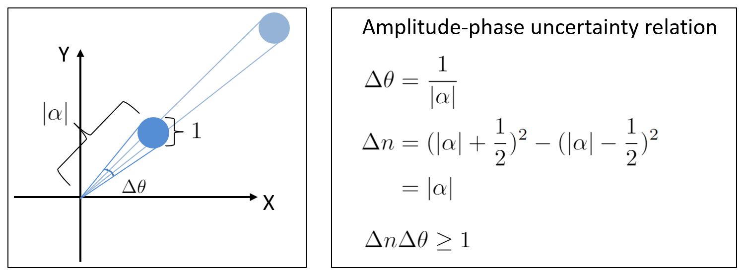
在相空间中,相干态是一个标准差为 1 的高斯函数。简单的几何学可以推导出粒子数-相位不确定性原理。
5.2.3 NOON 态
$|\Psi_0\rangle = \frac{|N\rangle \otimes |0\rangle + |0\rangle \otimes |N\rangle}{2}$
在 NOON 态中,我们实际上引入了一个 ancilla (辅助)系统,并将探针态和 ancilla 纠缠起来:当探针有 n 个光子时,ancilla 有零个光子;反之亦然。此时整体的哈密顿量为 $\hat{N} \otimes \mathbb{I}$。
此时量子 Fisher 信息为:
$F(\theta) = 4 [ \langle \Psi_0 | (\hat{N} \otimes \mathbb{I})^2 | \Psi_0 \rangle - \langle \Psi_0 | \hat{N} \otimes \mathbb{I} | \Psi_0 \rangle^2 ] = N^2$。
与相干态不同,NOON 态能够达到海森堡极限 $\Delta \theta = \frac{1}{N}$。选取观测量为 $N_X + iN_Y$,其中 $N_X = |+ \rangle\langle +| - |-\rangle\langle - |$,$N_Y = |+i \rangle\langle +i| - |-i\rangle\langle -i |$,且 $|\pm\rangle = \frac{|N\rangle \otimes |0\rangle \pm |0\rangle \otimes |N\rangle}{\sqrt{2}}$,$|\pm i\rangle = \frac{|N\rangle \otimes |0\rangle \pm i |0\rangle \otimes |N\rangle}{\sqrt{2}}$。请读者验证该观测量的期望值为 $e^{iN\theta}$,方差为 1,于是有 $1=|\Delta e^{iN\theta}| = |iN e^{iN\theta} \Delta \theta| = N\Delta \theta$,即 $\Delta \theta = \frac{1}{N}$,达到了海森堡极限。
然而,NOON 态是很脆弱的,当 N 稍微大一些就会退相干。实验上还没有制备出 N>10 的 NOON 态。这是因为 NOON 态是类似于薛定谔的猫,当 N 较大时很快就会退相干。从这一点来看,NOON 态并不实用,还不如相干态。
5.2.4 压缩态
我不打算给出压缩态的显式公式。实际上,你不需要公式也能理解压缩态。见下图
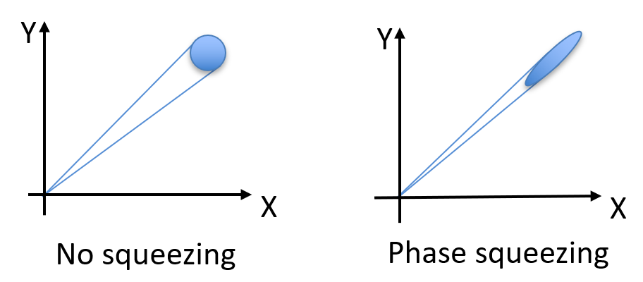
相位压缩
在相空间中,相干态是一个标准差为 1 的高斯函数。而压缩态其实就是将相干态在某一个 quadrature 上“压扁”了,从一个圆形变成了一个椭圆形。
压缩态仍然满足不确定性原理,只是在一个方向上的不确定性较大,在另一个方向上的不确定性较小。我们可以通过如上图所示的 Phase squeezing(相位压缩)来提高 $\Delta N$ 从而降低 $\Delta \theta$ 。反之,如果我们想要降低 $\Delta N$ ,我们可以通过提高 $\Delta \theta$ ,这就是 Amplitude squeezing(振幅压缩)。
振幅压缩态的 $g^{(2)}(0)<1$,而相位压缩态的 $g^{(2)}(0) > 1$ 。回想一下,我们有$(\Delta N)^2 = (g^{(2)}(0)-1)\langle \hat{N}\rangle^2 + \langle \hat{N}\rangle$ 。可见,对于压缩态, $\Delta N \propto \bar{n}$ , $\Delta \theta \propto \frac{1}{\bar{n}}$ ,达到了海森堡极限。压缩强度越大, $g^{(2)}(0)$ 就越大, $\Delta \theta \sim \frac{1}{k\bar{n}}$ 的比例系数 $k$ 就越高。
与脆弱的 NOON 态相比,压缩态更加实用一些。在文章开头我们就介绍过,著名的探测引力波的 LIGO 就使用了压缩态。另外,在样品损伤阈值较低的时候(例如生物样品),我们不能通过提高激光功率来降低散粒噪声,此时人们也使用压缩态来在不提升功率的前提下进一步提高成像精度。