光子的轨道角动量
前言
1992 年发表在 PRA 上的一篇文章 [1] 指出,光子也有轨道角动量(OAM,Orbital Angular Momentum)。与自旋角动量(即偏振,SAM,Spin Angular Momentum)只能取 $\pm \hbar$ 相比,轨道角动量可以取 $\hbar$ 的任意整数倍。这样的轨道角动量可以由螺旋形状的波前所携带。
你可能会惊奇:人们竟然到 1992 年才发现这件事情?实际上,早在 1992 年之前,螺旋形状的波前已经被人研究过;携带大于 $\hbar$ 的角动量的光子也早就已经被原子物理所预言(只不过它们来源于高阶跃迁过程,而高阶跃迁过程不满足选择定则,因此概率非常低,实验上基本没法观测)。直到 1992 年,Allen 等人才指出波前为螺旋形状的光束携带量子化的轨道角动量。
1992 年到 2001 年之间对 OAM 的研究基本处于宏观电磁波(大量光子的相干态)的范畴。诺奖得主 Zeilinger 组在 2001 年的一篇文章 [2] 中第一次研究了单个光子的轨道角动量及其纠缠。从此以后,OAM 也获得了量子信息和量子光学研究者们的兴趣。OAM 在量子信息中的一个可能的应用就是量子精密测量,这是因为它的 $e^{\mathrm{i}l\varphi}$ 因子有助于将角度测量的精度提升 $l$ 倍。另外,SAM 和 OAM 之间可以通过 q-plate 相互作用,有助于量子信息处理。OAM 还有许多其他经典应用 [3],这里就不赘述了。
一、Hermite-Gaussian (HG) 光束
在介绍携带轨道角动量的拉盖尔-高斯光束(Laguerre-Gaussian 光束)之前,我们最好先介绍埃尔米特-高斯光束(Hermite-Gaussian 光束)。
为什么要介绍高斯光束?因为实验上能得到的电磁波并不是理想平面波,而是激光器所输出的高斯光束。
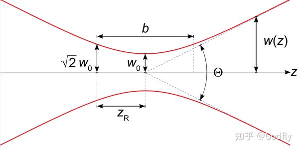
高斯光束的束腰宽度 w0、瑞利长度 zR 和发散角 theta,图源 Wikipedia
普通的埃尔米特-高斯光束的电场强度大小如下:
$\begin{aligned} E_{m,n}(x,y,z) = & ,E_0 \color{blue}{ \frac{w_0}{w(z)}\exp\left[-\frac{x^2+y^2}{w(z)^2}\right] } \times \\ & \color{green}{\exp\left[-\mathrm{i}\frac{k(x^2+y^2)}{2 R(z)}\right]} \color{orange}{\exp\left[\mathrm{i}\psi(z)\right]} \color{gray}{\exp[-\mathrm{i}kz]} \times \\ & \color{red}{H_m\left[\sqrt{2}\frac{x}{w(z)}\right]H_n\left[\sqrt{2}\frac{y}{w(z)}\right]} \end{aligned} $
其中:
$\color{blue}{w(z) = w_0 \sqrt{1+\left(\frac{z}{z_R}\right)^2}}$ 代表 $z$ 处的波束宽度, $z_R = \pi\frac{w_0^2}{\lambda}$ 是瑞利长度(Rayleigh length),定义为波束宽度发散到束腰宽度的 $\sqrt{2}$ 倍时的 $z$ 值。
$\color{green}{R(z) = \frac{z^2 + z_R^2}{z}}$ 代表 $z$ 处波前的曲率半径。
$\color{orange}{\psi(z)=\arctan\left(\frac{z}{z_R}\right)}$ 代表古伊相移(Gouy phase shift)。从负无穷远到正无穷远一共有 $\pi$ 的额外相移。
$\color{red}{H_m(t)}$ 是 $m$ 阶埃尔米特多项式。它们也是量子谐振子的能量本征解。当 $m,n$ 都等于零时,退化为基模高斯光束。大部分激光器输出的都是基模高斯光束。
可见,记忆高斯光束并不难,只要记住三个特征: $\color{blue}{\text{束腰发散}}$ 、 $\color{green}{\text{曲率半径}}$ 、 $\color{orange}{\text{古伊相移}}$ ,即可。
还有一个比较有用的量是发散角。从 $\color{blue}{w(z) = w_0 \sqrt{1+\left(\frac{z}{z_R}\right)^2}}$ 中可以看出发散角的正切值为 $\tan \theta=\frac{w_0}{z_R}$ ,于是有 $w_0 \tan \theta = \frac{\lambda}{\pi}$ 。
高斯光束的形状完全由波长、束腰半径、发散角三个中的任意两个决定。这三者之间的关系已经由 $w_0 \tan \theta = \frac{\lambda}{\pi}$ 给出。
$E_{m,n}(x,y,z)$ 只表示电场强度的大小,并未包含偏振信息。
加上偏振信息是很容易的:如果是 $x$ 方向偏振,只需要将 $E_{m,n}(x,y,z)$ 乘以 $x$ 方向的单位向量 $\hat{x}$ 即可。如果是圆偏振,只要乘以 $\hat{x} \pm \mathrm{i}\hat{y}$ 即可。
注意到 $E_{m,n}(x,y,z)$ 是一个复数。对于经典电磁波而言,真正的电场强度是它的实部。对于量子电磁波而言,我们可以指定该模式上的一个湮灭算符,这个湮灭算符是平面波湮灭算符的线性组合,系数可以由傅里叶分析得到。
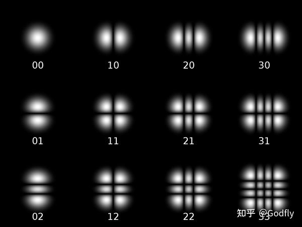
HG 模式,图源 Wikipedia
二、Laguerre-Gaussian (LG) 光束
在二维量子谐振子的解中,除了 Hermite 多项式所代表的线性振动以外,还有 Laguerre 多项式所代表的旋转运动。
下面我们给出拉盖尔-高斯光束的形式:
$\begin{aligned} E_{l,p}(r,\varphi,z) = & ,E_0 \color{blue}{ \frac{w_0}{w(z)}\exp\left[-\frac{r^2}{w(z)^2}\right] } \times \\ & \color{green}{\exp\left[-\mathrm{i}\frac{kr^2}{2 R(z)}\right]} \color{orange}{\exp\left[\mathrm{i}\psi(z)\right]} \color{gray}{\exp[-\mathrm{i}kz]} \times \\ & \color{red}{\left(\sqrt{2}\frac{r}{w(z)}\right)^{|l|} L_p^{|l|} \left(2 \frac{r^2}{w(z)^2}\right) \exp(-\mathrm{i}l\varphi)} \end{aligned} $
其中 $\color{blue}{\text{束腰发散}}$ 和 $\color{green}{\text{曲率半径}}$ 与埃尔米特-高斯光束相同,不同的有两点:
第一,高阶项由埃尔米特多项式变为拉盖尔多项式 $\color{red}{L_p^{|l|} (t)}$ 。且额外的因子 $\color{red}{\left(\sqrt{2}\frac{r}{w(z)}\right)^{|l|}}$ 和 $\color{red}{\exp(-\mathrm{i}l\varphi)}$ 分别表示原点处的奇点以及螺旋形的波前(带轨道角动量 $\hbar l$ )。
第二,古伊相移 $\color{orange}{\psi(z) = (2p + |l|+ 1)\arctan \frac{z}{z_R}}$ 变为 HG 模式的 $2p + |l|+ 1$ 倍。
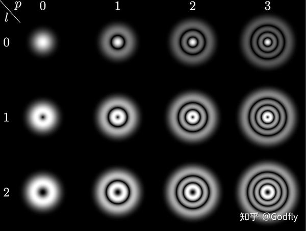
LG 模式,图源 Wikipedia
正如旋转可以分解为振动的线性叠加,LG 模式也可以表示为 HG 模式的相干叠加。这和圆偏振可以分解为两个线偏振的叠加类似。
三、用 Q-Plate 操控自旋角动量和轨道角动量
2006 年提出的 q-plate [4]本质上就是一个光轴与位置有关的半波片,且光轴的角度 $\alpha$ 满足 $\alpha(r,\varphi) = q \varphi + \alpha_0$ 。其琼斯矩阵为 $\begin{bmatrix} \cos 2\alpha & \sin 2\alpha \\ \sin 2\alpha & -\cos 2\alpha \end{bmatrix}$ 。
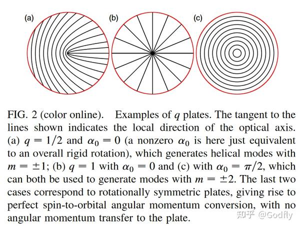
q-plate 的光轴图案,图源 [4]
考察一个 q-plate 作用到一个左旋偏振的基模高斯光束上,结果为:
$\begin{bmatrix} \cos 2\alpha & \sin 2\alpha \\ \sin 2\alpha & -\cos 2\alpha \end{bmatrix} \begin{bmatrix} \frac{1}{\sqrt{2}} \\ \frac{\mathrm{i}}{\sqrt{2}} \end{bmatrix} = e^{\mathrm{i}2q\varphi} \begin{bmatrix} \frac{1}{\sqrt{2}} \\ -\frac{\mathrm{i}}{\sqrt{2}} \end{bmatrix}$
可见,经过 q-plate,左旋偏振光变为带 $2q\hbar$ 轨道角动量的右旋偏振光。
q-plate 是目前实验上制备 OAM 态最常用的方法。当然,用 SLM 也可以。
OAM 之所以吸引量子信息研究者的兴趣,其中一个原因是它的希尔伯特空间维数和谐振子一样是无穷大的,而不像偏振(SAM)那样只有两个。SAM 与 OAM 之间的相互作用引出了一个很直接的想法:利用 SAM 和 OAM 做一个 CNOT 门,其中 SAM 是控制比特,OAM 是目标比特。类似的实验很多,这里就不放文献了。
参考
- Allen, L.; Beijersbergen, M. W.; Spreeuw, R. J. C.; Woerdman, J. P. Orbital Angular Momentum of Light and the Transformation of Laguerre-Gaussian Laser Modes. Phys. Rev. A 1992, 45 (11), 8185–8189. https://doi.org/10.1103/PhysRevA.45.8185.
- A. Mair, A. Vaziri, G. Weihs, and A. Zeilinger, “Entanglement of the orbital angular momentum states of photons,” Nature 412(6844), 313–316 (2001).
- Padgett, M. J. Orbital Angular Momentum 25 Years on [Invited]. Opt. Express 2017, 25 (10), 11265. https://doi.org/10.1364/OE.25.011265.
- Marrucci, L.; Manzo, C.; Paparo, D. Optical Spin-to-Orbital Angular Momentum Conversion in Inhomogeneous Anisotropic Media. Phys. Rev. Lett. 2006, 96 (16), 163905. https://doi.org/10.1103/PhysRevLett.96.163905.