【量光实验杂谈·一】非光子数分辨探测器测二阶关联函数(g2)的原理
HBT 实验
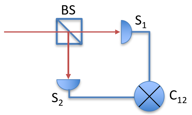
做量光实验的小伙伴一定知道 HBT 实验可以用来测二阶关联函数 g2,即将一束光用 50:50 的分束器分成两束,再分别用两个探测器探测,并统计两边光强的关联随延迟的变化,如下图所示:
Hanbury Brown and Twiss Experiment
经典 normalized g2 的定义为
$\begin{aligned} g^{(2)}(r_1,r_2;\tau)&=\frac{\langle E^*(r_1,t)E^*(r_2,t+\tau) E(r_2,t+\tau)E(r_1,t)\rangle}{\langle |E(r_1,t)|^2\rangle\langle |E(r_2,t+\tau)|^2\rangle} \\ &= \frac{\langle I(r_1,t)I(r_2,t+\tau)\rangle}{\langle I(r_1,t)\rangle\langle I(r_2,t+\tau)\rangle} \end{aligned}$
其中 $E$ 代表电场, $I$ 代表光强。可见,根据定义,HBT 实验测量的就是经典 g2(将关联光强除以两边各自的光强的乘积即可)。
量子二阶光联函数
量子 normalized g2 的定义为:
$\begin{aligned} g^{(2)}(r_1,r_2;\tau)&=\frac{\langle E^-(r_1,t)E^-(r_2,t+\tau) E^+(r_2,t+\tau)E^+(r_1,t)\rangle}{\langle E^-(r_1,t)E^+(r_1,t)\rangle\langle E^-(r_2,t+\tau)E^+(r_2,t+\tau)\rangle} \end{aligned}$
Comment:对于量子情况,分子里的算符要换成电场的 Counter-rotating Term $E^-$ 和 Co-rotating Term $E^+$ ,它们分别含有产生和湮灭算符。
而且,产生算符一定要在湮灭算符前面,因为一个光子被探测是一个湮灭的过程,这和经典情况不同。经典情况的相干态 $|\alpha\rangle$ 是湮灭算符的本征态 $a|\alpha\rangle=\alpha|\alpha\rangle$ ,多一个光子少一个光子没有什么区别。
在单模的情况下,由于 $E^+=i\sqrt{\frac{\hbar \omega}{2\epsilon_0 V}}a$ , $E^-=i\sqrt{\frac{\hbar \omega}{2\epsilon_0 V}}a^\dag$ ,于是量子 g2 可以化简为
$\begin{aligned} g^{(2)}(r_1,r_2,\tau)&=\frac{\langle a^\dag(r_1,t)a^\dag(r_2,t+\tau)a(r_2,t+\tau)a(r_1,t)\rangle}{\langle n(r_1,t)\rangle\langle n(r_2,t+\tau) \rangle} \end{aligned}$
于是,为了测量子 g2,我们要把光强探测器换成光子探测器,并且这个光子探测器可以分辨光子数。
然而问题来了,目前可以分辨光子数的单光子探测器都不太行:TES 回复时间太长;空间和时间上 Demultiplex 的方案只是伪光子数分辨;而 SNSPD 又很昂贵,需要低温,且多光子效率也未必很高。
NPNR-SPD 测 g2
幸运的是,不能分辨光子数的单光子探测器(NPNR-SPD,Non-Photon-Number-Resolving Single-Photon-Detectors)也可以测 g2,即使它们不能分辨光子数!
Comment:所谓“不能分辨光子数”的意思,就是它们只能区分“没有光子”和“有一个或多个光子”两种情况。常见的 APD 探测器就不能分辨光子数。
方法很简单:只要让 NPNR-SPD 的量子效率足够低就可以!
所谓量子效率 $\eta$ ,就是在有一个光子进入探测器的前提下,探测器能探测到这个光子的概率。反过来,这个光子被“损耗”掉的概率就是 $1-\eta$ 。
一开始我觉得很奇怪,怎么会效率越低越好呢?但是只要稍微想一想,就能明白其中原理:
当效率足够低的时候, $k$ 个光子没有全部被损耗掉的概率是 $1-(1-\eta)^k\approx k\eta$ ,也就是说 NPNR-SPD 探测到光子的概率正比于 $k$ 。这样,我们就通过“低效率”变相实现了“光子数分辨”。
下面是正式(无聊)的数学推导,可以跳过:
设探测器 1 的计数率为 $S_1$ ,探测器 2 的计数率为 $S_2$ ,两个探测器的符合(同时探测到光子的)计数率为 $C_{12}$ ,单位时间内光束里的光子数为 $R$ ,则有:
$\begin{aligned} S_i &=R\sum_{n=1}^{\infty}\frac{P_n}{2^n}\sum_{k=1}^{n}C_n^k[1-(1-\eta)^k] \\ &\approx R \sum_{n=1}^{\infty}\frac{P_n}{2^n}\sum_{k=1}^{n}C_n^k\cdot k\eta \\ &= R\frac{\eta}{2} \sum_{n=1}^{\infty} n P_n \end{aligned}$
$\begin{aligned} C_{12}&=R\sum_{n=1}^{\infty}\frac{P_n}{2^n}\sum_{k=1}^{n-1} C_n^k[1-(1-\eta)^k][1-(1-\eta)^{(n-k)}] \\ &\approx R \sum_{n=1}^{\infty}\frac{P_n}{2^n}\sum_{k=1}^{n}C_n^k\cdot k\eta \cdot (n-k)\eta \\ &= R \frac{\eta^2}{4} \sum_{n=2}^{\infty} n(n-1)P_n \end{aligned}$
于是
$\begin{aligned} \frac{C_{12} R}{S_1 S_2} &= \frac{\sum_{n=2}^{\infty} n(n-1)P_n }{\left(\sum_{n=1}^{\infty} n P_n\right)^2} \\ &= \frac{\langle n(n-1) \rangle}{\langle n\rangle^2} \end{aligned}$
熟悉量子光学的人应该已经看出这就是 g2 了。推导如下:
$\begin{aligned} g^{(2)}(r_1,r_2,\tau)&=\frac{\langle a^\dag(r_1,0)a^\dag(r_2,\tau)a(r_2,\tau)a(r_1,0)\rangle}{\langle n(r_1)\rangle\langle n(r_2) \rangle} \end{aligned}$
令 $r_1=r_2,\quad \tau=0$ 得
$\begin{aligned} g^{(2)}(\tau=0)&=\frac{\langle a^\dag a^\dag a a \rangle}{\langle n\rangle^2} \\ &= \frac{\langle a^\dag(aa^\dag -1) a\rangle}{\langle n\rangle^2} \\ &= \frac{\langle n^2-n\rangle}{\langle n\rangle^2} \end{aligned}$
测 g2 有什么用呢?除了教科书里常见的区分【超泊松统计/泊松统计/亚泊松统计】以及区分【光子集聚/反集聚】以外,还有一个意想不到的作用:测量光子的频谱关联。下篇我们就来讨论这一点。
尾声:多模情况
前面我们埋下了一个小伏笔:我们假设了被探测光是单模的。于是 $E^+$ 可以正比于 $a$ : $E^+=i\sqrt{\frac{\hbar \omega}{2\epsilon_0 V}}a$ 。
但如果被探测光是多模的会如何?此时 $E^+=i\sum_{k}\sqrt{\frac{\hbar \omega_k}{2\epsilon_0 V}}a_k$ ,$E^+$ 不再正比于 $a$ 了,而是有一个频率依赖: $E^+_k\propto \sqrt{\omega_k}a_k$ 。
由于原本的 g2 探测的是光强,而光强等于 频率乘以光子数,因此这里有一项 $\sqrt{\omega_k}$ 是不奇怪的。
不过只要各个模式的频率相同,我们还是可以约掉 $\sqrt{\omega_k}$ ,得到:
$\begin{aligned} g^{(2)}(0)=\frac{\left\langle :\left(\sum_k a^\dag_k a_k\right)^2:\right\rangle}{\left\langle \sum_k a^\dag_k a_k\right\rangle^2} \end{aligned}$
其中 $::$ 代表正规排序,即将所有产生算符都移到湮灭算符的前面。
令 $n=\sum_ka^\dag_k a_k$ ,有
$\begin{aligned} g^{(2)}(0)=\frac{\langle n(n-1)\rangle}{\langle n\rangle^2} \end{aligned}$
可见,虽然有多个模式存在,但如果这些模式的频率(近似)相同,那么 HBT 实验测量量子 g2 的方法仍然是有效的。